Table of Contents
- Attention
- This tutorial is currently under construction. The figures do not reflect the parameters documented, as these parameters will be finalized soon.
This tutorial aims to replicate the passive mixer problem by C. S. Andreasen et al. 2009.
The goal of this optimization problem is to design a structure capable of mixing fluids in a static manor, that is to say, without the use of moving parts.
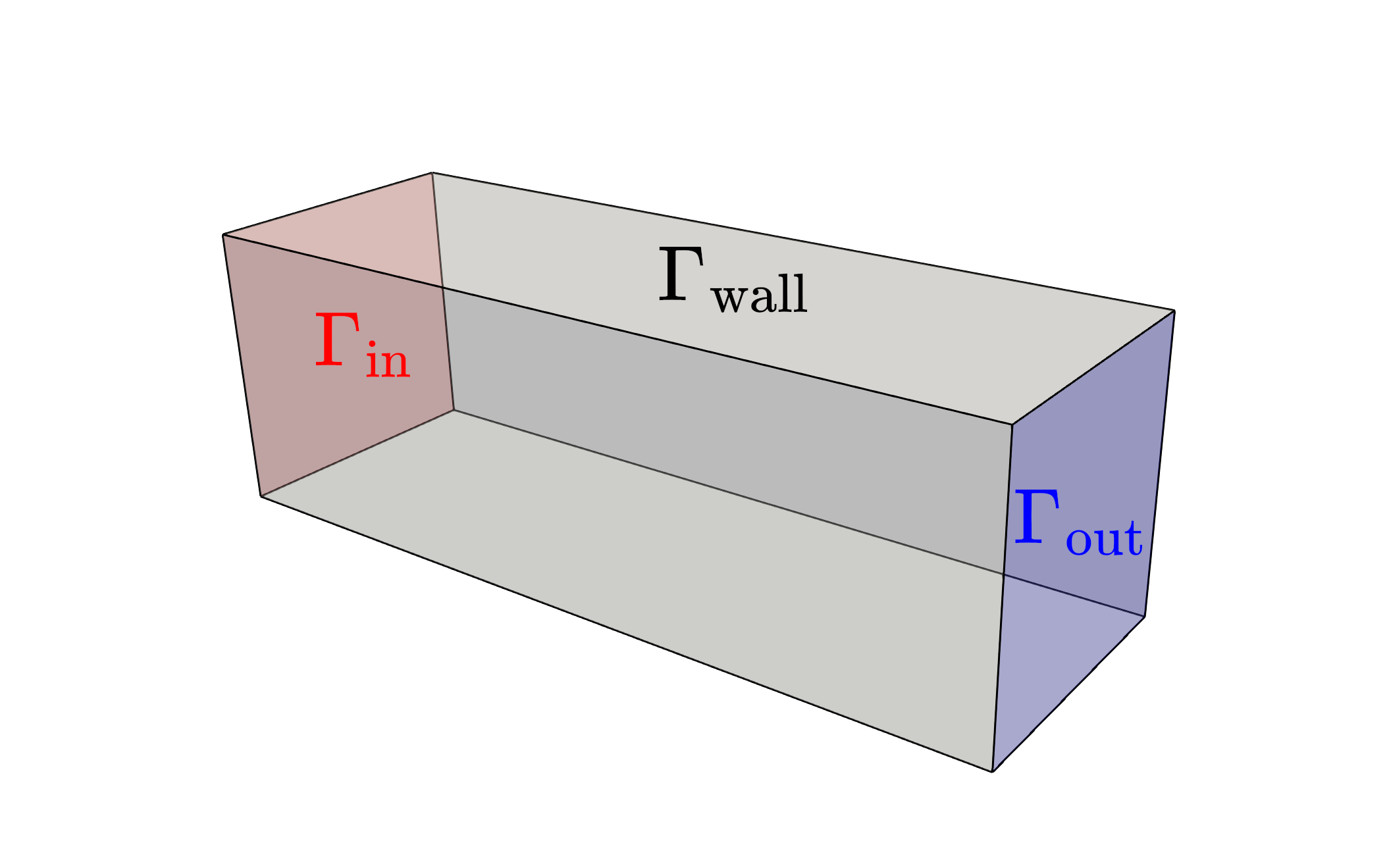
We begin by considering a square duct seen in the figure below.
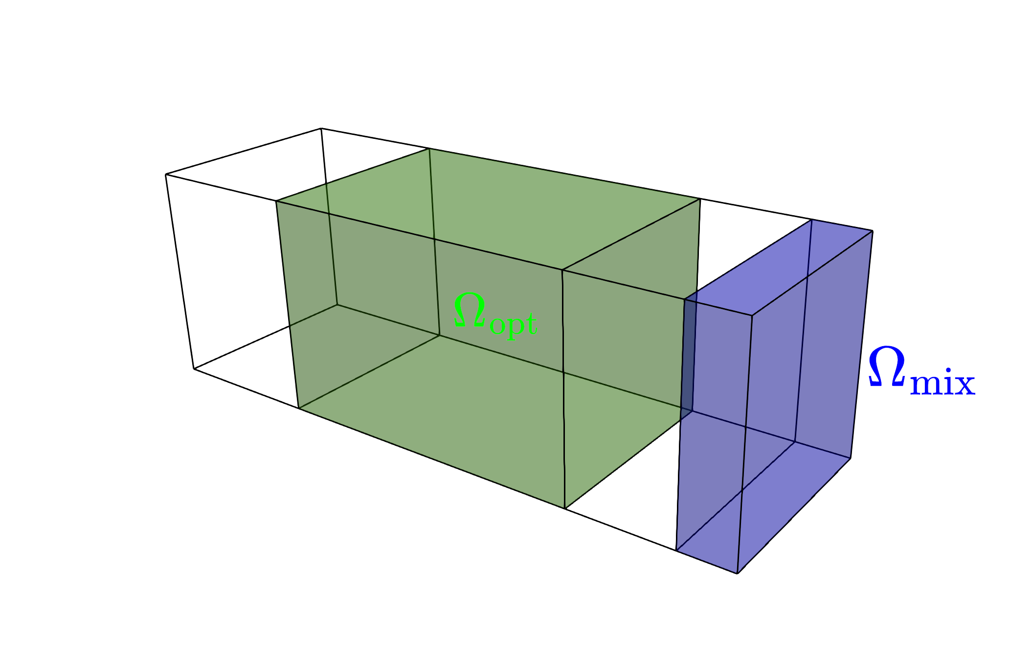
Fluid enters the domain upstream and is ejected downstream, with all other boundary being considered solid walls. In addition, we consider a scalar field, representative of the two species one desires to have mixed (denoted in red and blue in the above figure). The species enters the mixer upstream, originally separated into two distinct species. The goal of the optimization problem is to design the interior structure such that the two species are as homogeneous as possible in the downstream location (denoted in green in the above figure). The system is assumed to be low Reynolds number, implying a steady state solution can be found, and high Peclet number, implying the mixing must be performed by advective transport, not diffusion.
In this tutorial you will learn how to
- Formally define this problem in the context of a topology optimization problem.
- Mesh the domain.
- Set up a fluid, scalar and their respective adjoint simulations.
- Define different domains
- Define the objective functions and constraints being solved.
- Define a mapping cascade.
- Define parameters for the optimization algorithm.
- Prepare a driver to solve the optimization problem.
- Solve the optimization problem.
- Post process the results.
Defining the optimization problem
We define the duct as the domain \(\Omega\). The equations being solved in \(\Omega\) are the incompressible Navier-Stokes equations with an additional passive scalar equation
\[ {\frac {\partial \mathbf {u} }{\partial t}} + (\mathbf {u} \cdot \nabla)\mathbf {u} = -\nabla p +{\frac {1}{Re}}\nabla ^{2}\mathbf {u} + \mathbf{f} - \chi \mathbf{u}, \\ \nabla \cdot \mathbf {u} = 0, \\ {\frac {\partial \phi }{\partial t}} + (\mathbf {u} \cdot \nabla)\phi = {\frac {1}{Pe}}\nabla ^{2}\phi ,\\ \]
subject to boundary conditions
\[ \frac{1}{Re} \nabla \mathbf{u} \cdot \mathbf{n} -p \mathbf{n} = 0, \text{ on } \Gamma_\text{out}, \\ \mathbf{u} = \mathbf{u}_\text{in}, \text{ on } \Gamma_\text{in}, \\ \mathbf{u} = \mathbf{0} \text{ on } \Gamma_\text{wall}, \\ \nabla \phi \cdot \mathbf{n} = 0, \text{ on } \Gamma_\text{out} \cup \Gamma_\text{wall}, \\ \phi = \phi_\text{in} \text{ on } \Gamma_\text{in}, \\ \]
where \(\mathbf {u}(\mathbf{x},t)\) denotes the velocity field, \(p(\mathbf{x},t)\) the pressure field, \(\mathbf{f}\) a forcing term, \(\phi(\mathbf{x},t)\) the scalar field and where \(Re\) and \(Pe\) denotes the Reynolds and Peclet numbers respectively. Here, \(\chi(\mathbf{x})\) is a Brinkman penalization term used to impose the presence of material within the domain and acts as a simplified Immersed Boundary Method (IBM) proposed by Goldstein. That is, \(\chi\) is the spatially dependent Brinkman coefficient, satisfying
\[ \chi = \begin{cases} 0 & \text{in the fluid region,} \\ \overline{\chi} & \text{in the solid region,} \end{cases} \]
where it is assumed that \(\overline{\chi}\) to be a large value, resulting in a forcing term that models a momentum loss in solid region. We also define two domains, an optimization domain \(\Omega_\text{opt} \subset \Omega\) in which we can place material and a domain downstream in which we want the scalar species to be mixed \(\Omega_\text{mix} \subset \Omega\).
We can now define our objective function to be minimized as
\[ \mathcal{F} = \frac{1}{|\Omega_\text{mix}|}\int_{\Omega_\text{mix}} \frac{1}{2} (\phi - \phi_\text{ref})^2 d\Omega, \]
where \( \phi_\text{ref} \) is a target reference concentration and \( |\Omega_\text{mix}| \) denotes the volume of the the domain \( \Omega_\text{mix} \).
- Note
- In the original paper by C. S. Andreasen et al. 2009 they also constrained this optimization problem with a pressure drop constraint. This functionality is still in the process of being implemented into
neko-top.
We now introduce the abstract material indicator \(\rho(\mathbf{x})\), where \(\rho = 1\) denotes the presence of solid material, while \(\rho=0\) denotes the absence of material. The material indicator should ideally take discrete values, however, following a density-based approach, we allow for intermediate values \(\rho \in [0,1]\). This avoids an integer-valued optimization problem and allows gradient-based optimization techniques. A discussion on the mapping \( \rho \mapsto \chi\) is left for Mapping cascade.
Finally we can cast our optimization problem as
\[ \underset{\rho}{\text{min }} \mathcal{F},\\ \text{subject to:} \\ \text{Governing equations}, \\ \text{Boundary conditions.} \]
Given this optimization consists of a single objective function and an exhaustively large number of design variables, it is natural to solve this problem with adjoint based sensitivity analysis and gradient decent algorithms.
The remained of this tutorial will guide you through the process of solving such an optimization problem with the topology optimization framework neko-top.
prepare.sh and meshing
neko-top provides users with the capability of executing custom scripts before an the simulation begins but including a prepare.sh script in the example folder. This functionality is commonly used to generate meshes or other preprocessing steps.
An extensive review of the meshing tools available in neko and neko-top can be found in Meshing. In this tutorial we will be utilizing the neko utility genmeshbox in the prepare.sh script to generate \( \Omega \) from a cartesian mesh. The key excerpts in this script read
indicating that a box mesh of dimensions \([0,6] \times [0,2] \times [0,2] \) will be created with \(30 \times 10 \times 10 \) elements.
- Note
- The
.false.arguments refer to periodic boundary conditions, which innekoare treated as topologically linking these boundary. In the current problem there are no periodic boundary conditions, hence the.false.arguments
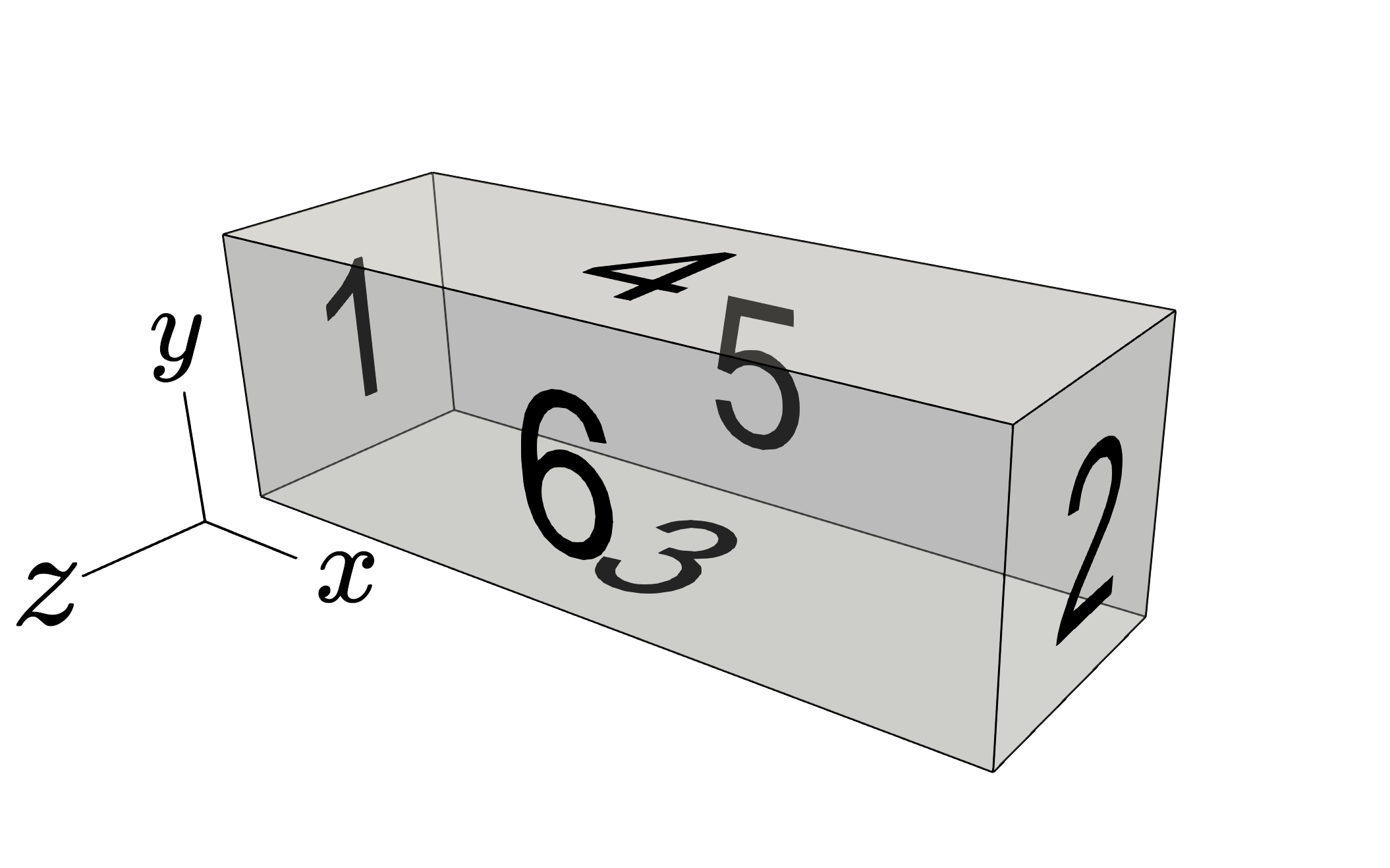
An important consideration when using genmeshbox is the boundary identifiers, which become relevant when prescribing boundary conditions. The convention is to label from 1-6 in the order \([x_\text{start}, x_\text{finish}, y_\text{start}, y_\text{finish}, z_\text{start}, z_\text{finish}] \) or as indicated in the figure below.
The neko-top .case file
The *.case file allows the user to set up the case. The high level case structure is described extensively in the neko documentation which can be found here. The reader is strongly encouraged to refer to this documentation in regards to setting up a forward simulation. In neko-top, the high level case structure is extended to allow for additional adjoint and optimization parameters. The neko-top high level case structure reads
Case
The top level of the case file allows the user to prescribe details on the numerics and case set up.
- Note
- The default name when using
genmeshboxis"box.nmsh".
It is common practice in neko-top to disable the inbuilt neko file outputs, and instead rely on the output samplers provided by neko-top to alleviate excessive outputs when looping between the forward and adjoint runs.
Here we have prescribed:
- a time-step \(\Delta t = 2\times 10^{-4} \) (
"timestep": 2e-4) - a first order time integration scheme (
"time_order": 1) - a polynomial order of 6 (
"polynomial_order": 6) - the use of overintegration when evaluating the convective terms (
"dealias": true)
- Attention
- Despite intending to solve the steady Navier-Stokes equation, Currently an
end_timemust be prescribed inneko. More details regarding steady state solutions can be found in Simulation components but there are intentions to include steady state functionality directly withinneko, streamlining this process.
Instead, steady states are currently marched towards using the the steady state simulation component
- Attention
- Currently certain features of
nekoare not supported byneko-topdue to a lack of adjoint support. Relevant to this section, it should be noted that variable time-stepping is not supported.
Fluid
The fluid section of the case file allows the user to prescribe fluid properties, solvers, boundary conditions and initial conditions.
The key details which are prescribed are:
- a significantly low Reynolds number (
"Re": 2) - an initial \( \mathbf{u}|_{t=0} = \mathbf{0}\)
- no slip boundary conditions on \(\Gamma_\text{wall}\)
- an outflow boundary condition on \(\Gamma_\text{out}\)
- a user defined inflow condition on \(\Gamma_\text{in}\)
- Note
- The velocity and pressure solvers have been set relatively conventionally, however the interested reader can find more information here.
- Attention
- It should be noted that some features in
nekoare not supported inneko-topdue to a lack of adjoint support. Relevant to this section, it should be noted that the use of projections or gradient jump penalty are not supported.
To prescribe user defined conditions, such as the condition on \(\Gamma_\text{in}\) users can provide additional fortran code. In this tutorial we will provide an additional user.f90. Further details on the neko user interface can be found here.
In this tutorial we wish to prescribe a paraboloid as an inflow condition, this is achieved by asserting userfluid_user_if => user_inflow_eval and providing the following code excerpt:
Scalar
Similarly, the scalar section of the case file allows the user to prescribe scalar properties, solvers, boundary conditions and initial conditions.
The key details which are prescribed are:
- a significantly high Peclet number (
"Pe": 5000.0) - a user defined initial condition
- Neumann conditions on \( \Gamma_\text{out} \cup \Gamma_\text{wall} \)
- a user defined scalar inflow condition on \( \Gamma_\text{in}\)
The user defined scalar inflow condition and scalar initial condition are prescribed with userscalar_user_bc and userscalar_user_ic. Here we wish to prescribe a separation between the two scalar species where \(\phi = 0\) represents one species and \(\phi = 1\) represents the other. It is well understood that spectral methods struggle to represent discontinuities, hence, a sigmoid function is use to provide a sufficient amount of smoothing across the interface of the two species. The completed user.f90 should now read:
Adjoint fluid and scalar
This tutorial will focus on the practical aspects of setting up the adjoint simulation however the theory regarding adjoint sensitivity analysis can be found in Adjoint sensitivity analysis.
- Note
- An important feature to be aware of in the
neko-topadjoint system is that unless a parameter is specified, the adjoint will adopt the same parameters as their primal counterparts. For instance, by not specifying a solver type for the adjoint fluid,neko-topwill use the same solver types used in the fluid.
The key details which are prescribed are:
- \( \phi^\dagger = 0\) on \( \Gamma_\text{in} \)
- \( \nabla \phi^\dagger \cdot \mathbf{n} = 0\) on \( \Gamma_\text{out} \cup \Gamma_\text{wall} \)
- \( \mathbf{u}^\dagger = \mathbf{0}\) on \( \Gamma_\text{in} \cup \Gamma_\text{wall} \)
- an outflow velocity boundary condition on \( \Gamma_\text{out} \)
Domain specification
Domains can be specified through the neko functionality point_zones, the reader is referred here for extensive documentation on point zones.
In this tutorial we must define \(\Omega_\text{opt}\) and \(\Omega_\text{mix}\) which we name optimization_domain and objective_domain respectively.
Assigning \(\Omega_\text{opt}\) to the optimization domain is performed in the optimization section of the case file
Objectives and constraint
Various objectives and constraints can be provided as lists in the objectives and constraints subsection of optimization. A full list of the available objectives and constraints can be found in Objectives and constraints.
- Attention
- In the future we wish to also include a tutorial teaching users how to implement their own custom objectives and constraints, however this is yet to come.
In this tutorial we wish to assign a "scalar_mixing" objective and no constraints by prescribing
In neko-top multiple objectives can be prescribed in a list, resulting in a multi-objective optimization problem which is handled by a weighted sum of all prescribed objectives
\[ \mathcal{F} = \sum_i w_i \mathcal{F}_i, \]
where \(w_i\) is a prescribed weight.
Multiple constraints on the other hand are also entered in a list but are handled through the MMA functionality discussed in The Method of Moving Asymptotes (MMA).
Since the scalar \( \phi \in [0,1]\), we set a target value for the scalar concentration to \( \phi = 0.5\) ("phi_ref": 0.5) and assert the area of interest is in \( \Omega_{mix}\) ("mask_name": "objective_domain").
Mapping cascade
We saw in Defining the optimization problem that the design indicator field \(\rho\) must be mapped to the Brinkman amplitude \(\chi\). This is achieved through the use of the mapping cascade accessible in optimization.design.mapping. A detailed description of the mapping cascade and available mappings in neko-top can be found in Mapping cascade.
In this tutorial we use the composite mapping \(\rho \mapsto \tilde{\rho} \mapsto \chi\) where
- \(\rho \mapsto \tilde{\rho} \) is a spatial filter
- \(\tilde{\rho} \mapsto \chi\) is a RAMP mapping
which can be prescribed with
- Note
- It is important to note that the order in which the mappings occur in the case file is the order in which they will be executed.
Here we have prescribed a spatial filter with radius 1 followed by a RAMP mapping with maximum Brinkman amplitude 1000.
The mapping cascade takes care of both mapping the design forward and performing the chain rule backward, i.e.
\[ \frac{\partial F}{\partial \chi} \mapsto \frac{\partial F}{\partial \tilde{\rho}} \mapsto \frac{\partial F}{\partial \rho} \]
Optimization parameters
The optimization algorithm used to solve optimization problem is prescribed in the "solver" section of the case file. Currently on the MMA algorithm is implemented and more details can be found in The Method of Moving Asymptotes (MMA).
In this tutorial we we select the MMA algorithm by prescribing
The key parameters selected are
- a maximum of 100 optimization iterations (
"max_iterations": 100) - a convergence criterion of 1.0e-3 (
"tolerance": 1.0e-3) - no constraints (
"m": 0) - a scaling factor of 1000 for the objective function (
"scale": 1000.0) - assert that \( \rho \in [0,1] \)
Scaling factors can be adjusted to influence convergence rates of the optimization problem.
The final case file
The final case file should now read
Neko-top drivers
neko-top exists as a library of tools to allow users to perform optimization in conjunction with the neko library. As such, the user has the freedom to create custom drivers to perform specific tasks. Further details regarding drivers can be found in Advanced example setups.
This functionality can be achieved by providing a driver.f90 file in the example folder along with a CMakeLists.txt.
For this tutorial, we provide the following CMakeLists.txt
This script performs the following task:
- allows
neko-topto use a custom driver (set(DRIVER_TYPE "custom")) - indicates to
neko-topto use thedriver.f90driver (set(DRIVER_SOURCE ${CMAKE_CURRENT_SOURCE_DIR}/driver.f90)) - includes the additional
user.f90file used to prescribe user boundary conditions and initial conditions.
neko-top distinguishes between four key objects:
- design. The design space over which one optimizes.
- problem. The definition of the optimization problem being solved.
- optimizer. The optimization algorithm used to solve the optimization problem.
- simulation. Specifically for problems involving fluid mechanics, a simulation can allow for interfaces with
nekoto perform forward simulation and additionalneko-toplibraries to perform adjoint sensitivity analysis.
Further details regarding these components can be found in Code structure .
The basic structure of driver.f90 is to
1) declare these objects
2) initialize these objects along with the user specified boundary and initial conditions
3) run the optimization algorithm
4) clean
The driver file
The complete driver takes the following form
Solving the optimization problem
Once the example has been constructed it can be run by simply executing
from the root neko-top directory. Further details on the functionality of the run script run.sh can be found in Examples.
Post processing the results
The output from a neko-top topology optimization problem consists of three key components
1) an optimization log, saved in the file optimization_data.csv. 2) a log of the steady state residual, saved in the file steady_state_data.csv. 3) a series of field files
- the steady state forward solution
forward_fields0.nek5000 - the steady state adjoint solution
adjoint_fields0.nek5000 - the design field
design0.nek5000
Within design0.nek5000 there are 3 fields labeled x_velocity, y_velocity and z_velocity, these fields correspond to:
x_velocity: The unmapped design field \(\rho \in [0,1]\)y_velocity: The mapped design field \(\chi \in [0,\chi_{\text{max}}]\)z_velocity: The sensitivity \(\partial \mathcal{F}/\partial\)
Included in this example is a folder passive_scalar/post_processing containing:
plot_convergence.py: A python script to plot the convergence historypost_processing.pvsm: A Paraview state file to assist you with visualizing the optimized designs.
- Attention
- The remainder of this tutorial is under construction, however it intends to help you understand how to process these files and provide some scripts to help you visualize the results.